3 Social Diffusion
This chapter introduces how behaviors spread through social learning and why this process is central to sustainability. We begin by framing behavior diffusion in terms of prevalence — the fraction of people in a population practicing a behavior — and show how different learning rules (contagion, conformity, success-bias) can be expressed within a single mathematical framework, the prevalence dynamic. We then show how to measure collective adaptation through outcome measures such as success rate and time to fixation, using computational experiments. Applications demonstrate how this framework clarifies the strengths and weaknesses of different learning rules, why conformity cannot drive adaptation by itself, and why minority groups play an essential role in sustainability. The chapter closes with a preview of diffusion in networks, setting the stage for the following chapter.
3.1 Introduction
Sustainable action, whether it is adopting renewable energy, changing agricultural practices, or reducing inequality, is ultimately a matter of how behaviors spread. Behaviors spread because people learn from one another. This process of social learning over time is the fundamental mechanism of collective adaptation.
Collective adaptation is represented in terms of the prevalence of a sustainable adaptation — the fraction of people in a population who practice the adaptive behavior. To quantify the effects of different social, cognitive, and ecological factors on adaptation prevalence we need a way to mathematically describe how people learn from each other over time.
3.1.1 Introducing The Prevalence Dynamic
The prevalence dynamic represents collective adaptation (or maladaptation) as the aggregation of individual-level behavior decisions. At its core, the prevalence dynamic tracks two probabilities: the chance that a person switches from the legacy behavior to the adaptive behavior (adoption probability) and the chance that a person switches back from the adaptive to the legacy behavior (drop probability). By combining these probabilities with the current prevalence of each behavior, we obtain a dynamic description of how behavior spreads in a population.
3.1.3 Model Implementations
Each learning model can be implemented in different mathematical ways, depending on how we represent the population and how much randomness we allow. These implementations are summarized in the next table.
| Implementation | Formalism | Population assumption | What it shows best | Limitation |
|---|---|---|---|---|
| Deterministic Prevalence Dynamic (DPD) | Differential equations | Large N, well-mixed | Mean-field dynamics; limiting cases | Ignores stochasticity and structure |
| Stochastic Prevalence Dynamic (SPD) | Markov / diffusion approximations | Finite N, well-mixed | Fixation probability; role of drift | Harder to solve analytically |
| Agent-based Prevalence Dynamic (APD) | Explicit agents and interactions | Any N; can include networks | Flexibility, heterogeneity, emergent dynamics | Computationally intensive; harder to generalize |
3.1.4 Chapter Overview
In Section 2, we introduce the prevalence dynamic, a simple way of describing behavior change over time in terms of math. We show how the same framework can capture different learning rules — contagion, success-biased learning, and conformity — by specifying their adoption and drop probabilities. These probabilities are written as functions of the current prevalence of each behavior, since learning requires others to be present who already practice the behavior and can serve as models. In this way, prevalence itself drives the dynamics.
In Section 3, we use these models to explore applications to sustainability. We begin with exemplary applications: comparing prevalence dynamics with different learning models, analyzing why conformity can only lead to fixation through drift, and extending the framework to cases with minority and majority groups. Even these simplified models provide important lessons: collective adaptation works best when people are educated to evaluate the benefits and risks of different behaviors; collective adaptation can never happen through conformity alone if adaptive behaviors are initially rare; and minority groups must be included as participants and highlighted as leaders in sustainability interventions. To understand more specific questions, like how social network structure affects diffusion, we will need additional techniques, which we take up in subsequent chapters.
The chapter closes by reflecting on what these different learning rules mean for promoting sustainable practices in the real world, emphasizing when and how social learning can help collective action succeed.
3.2 Prevalence Dynamic
The prevalence dynamics modeling framework provides a structure for various modeling choices one could make to represent social diffusion of behaviors. This framework includes explains which choices could be useful in which socio-ecological contexts. Sustainability provides social science an important challenge to identify principles that could predict how likely different sustainability interventions are to succeed, and to examine how the prevalence of sustainable behaviors change over time.
In this section I explain how this framework can address this challenge by first introducing the prevalence dynamic in a series of forms, starting with the mathematical form. Next in this section, I explain how to create agent-based models of social diffusion using socmod. The prevalence dynamic can be used to create quantitative models of behavior diffusion, generating simulated observations of the prevalence of behaviors over time. We also measure simulated outcomes of whether or not a simulated intervention was successful. Simulations count as successful if all or some large fraction of individuals adopt a sustainable adaptive behavior.
We will apply this framework to generate some important insights for intervention design in the following section, Applications. For now we start by explaining the structure of a social diffusion simulation by first sketching options for representing the social learning process, i.e., the social learning model. The prevalence dynamic is the foundation for quantitative simulations of individuals learning from others over a series of simulated time steps. Simulations can be implemented and analyzed with math or code, also explained in more detail below.
3.2.1 The Prevalence Dynamic
In these models we assume there are two possible behaviors, or classes of behaviors, that individuals can do. These are called the Adaptive behavior or practice, or behavior \(A\) for short. The non-adaptive or maladaptive behavior is the Legacy behavior, i.e., the business-as-usual behavior. An individual who does the adaptive behavior is an \(A\)-doer, and one doing the legacy behavior is an \(L\)-doer.
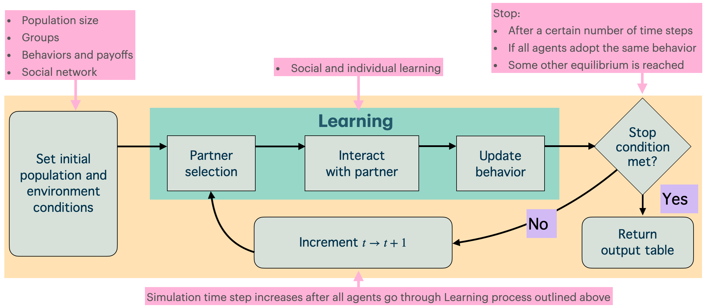
To represent interventions, we initialize agent populations with one behavior or the other, specify environmental or ecological conditions such as the apparent benefit of different behaviors, and set agent learning strategies. Learning strategies that we consider are contagion (probabilistic adoption on exposure), success-biased learning (successful individuals are more likely to be chosen as teachers), and conformity or frequency-biased learning (more prevalent behaviors are more likely to be adopted).
The model represents time in steps. On each time step, agents select partners, interact, and update behaviors based on outcomes and learning rules. These steps are repeated until specific conditions or thresholds are met. Stopping conditions are typically specified as when a maximum time step is reached, when the entire population fixates (i.e., all do the same) on one behavior or the other. After the model stops, the dynamics can be inspected or the outcomes can be aggregated across simulations in the case of agent-based modeling.
3.2.2 Formal models of diffusion
In the next chapter I explain how to develop various formal models of behavior diffusion that represent changes in prevalence of different behaviors.
Collective Adaptation through Individual Decisions
(EXPLAIN THE MODELING APPROACH, TAKING IT FROM THE INTRODUCTION)
Agent-based models of diffusion
Agent-based models (ABMs) provide a structured way to explore complex systems by simulating interactions between autonomous agents, i.e., simulated people. In sustainability contexts, ABMs offer a low-cost testbed for understanding how interventions might impact social dynamics and environmental outcomes. For example, Airoldi and Christakis (2024) demonstrated through regression analysis across that one method for selecting individuals targeted in a public health education campaign worked better than another. They studied over 20,000 individuals across Honduran villages of about 100 people each to reach their findings. Real-world verification of the efficacy of different intervention strategies is important. However, we can also use agent-based models to represent the diffusion of information in simulated populations where interactions are structured by model social networks. We can initialize thousands or millions of simulated villages in which this information could diffuse with different intervention strategies, and observe the distribution of the adoption of sustainable behaviors for each potential intervention strategy. We can then analyze which performed best in silico, which can be helpful if interventions will be taken to different contexts. In other worlds, we can use ABMs to deduce how different learning rules, group identities, and social structures shape sustainability outcomes generally, which can guide our selection of real-world intervention strategies.
We will analyze and draw on several real-world empirical studies of interventions to develop our agent-based models that we in turn will use to simulate interventions in order to deduce which strategies are most effective for social interventions to promote sustainability, and why. A social intervention (or just intervention) for promoting sustainability is any concerted effort where those promoting a sustainable practice introduces information about how to perform that practice to a population. Deductive methods complement regression-based inferential or inductive strategies. Deductive strategies can explain which strategies are most effective and why in idealized, cost-free settings (cost-free at least compared to the cost of real-world social interventions at scale).
Low-cost experimentation with simulated social interventions to promote sustainability are critical. Unless progress is accelerated towards we can expect to “have 575 million people living in extreme poverty, 600 million people facing hunger, and 84 million children and young people out of school. Humanity will overshoot the Paris climate agreement’s 1.5°C ‘safe’ guardrail on…temperature rise. And, at the current rate, it will take 300 years to attain gender equality” (Malekpour et al. 2023, 250). Accelerated transformations are required to reach goals necessary to avoid increasingly frequent and costly climate change disasters (United Nations 2023). It is not plausible to do real-world experiments at the global scale required to infer which strategies work best in which situations.
In this course we will focus on deducing how between different cognitive and social factors, or other initial conditions, affect simulated sustainability intervention outcomes. We will frame our studies in terms of sustainable development goals, but we will never fit our models to observations. Nonetheless, we will strive to develop models that are amenable to real-world interventions against which the models could be fit and predictions could be compared. It seems this is not done too much in practice yet in sustainability. However, some of our colleagues focused on studying basic processes that underlie cultural transmission do exactly this to explain experimental data and archaeological observations (Deffner et al. 2024), which thereby improves their theory, models, and understanding of cultural evolution in a theory-model-observation cycle. With more time and research effort, this cycle may become commonplace in sustainability.
The urgent need to understand how sustainable behaviors spread in order to develop effective interventions pressures social scientists to make social science more rigorous, reliable, and digestible by non-social scientists. In the rest of this Introduction we review cognitive and social theories of social learning, identity and influence, homophily and core-periphery network structures, and preview the remainder of the course material. For an overview of the course feel free to skip ahead to the Plan in table format.
Contagion
For contagion, adoption occurs when a legacy-doer encounters an adaptive-doer and switches with probability \(\alpha\), while dropping occurs when an adaptive-doer reverts to the legacy behavior with probability \(\delta\), regardless of prevalence.
Adoption probability:
\[ P(A \mid L) = \alpha a \]Drop probability:
\[ P(L \mid A) = \delta \]
Normalizing:
\[ P(A) = (1-a) P(A \mid L) + a P(A \mid A), \]
with \(P(A \mid A) = 1 - \delta\), we obtain the prevalence dynamic
\[ \dot a = \alpha a (1-a) - \delta a. \]
Success-biased Learning
Adoption depends on both prevalence and relative success.
Adoption probability:
\[ P(A \mid L) \propto a f_A \]Drop probability:
\[ P(L \mid A) \propto (1-a) f_L \]
Normalizing by total “success weight” \(\bar f = af_A + (1-a)f_L\):
\[ P(A) = \frac{a f_A}{\bar f}, \]
yielding the prevalence dynamic
\[ \dot a = \frac{a f_A}{\bar f} - a = \frac{a}{\bar f}(f_A - \bar f). \]
Conformity
Adoption depends on the relative prevalence of behaviors, weighted by conformity strength \(\gamma\).
Adoption probability:
\[ P(A \mid L) \propto a^{1+\gamma} \]Drop probability:
\[ P(L \mid A) \propto (1-a)^{1+\gamma} \]
Normalizing:
\[ P(A) = \frac{a^{1+\gamma}}{a^{1+\gamma} + (1-a)^{1+\gamma}}, \]
so the prevalence dynamic is
\[ \dot a = \frac{a^{1+\gamma}}{a^{1+\gamma} + (1-a)^{1+\gamma}} - a. \]
3.2.3 Measuring Collective Adaptation
To make sense of different learning models, we need to decide what to measure. The prevalence dynamic generates several observables: - Prevalence of adaptive behavior over time, \(a(t)\).
- Fitness or success values of behaviors, if defined (\(f_A\), \(f_L\)).
- Transition probabilities, such as \(P(A \mid L)\) and \(P(L \mid A)\).
From these observables, we define outcome measures that summarize how well an adaptive behavior spreads: - Success rate: the probability that the adaptive behavior eventually becomes common or dominant.
- Time to fixation (or last time step): how long it takes, if ever, for the adaptive behavior to be adopted by everyone.
Studying these outcomes requires what we call a computational experiment. A computational experiment specifies a learning model, population assumptions, and initial conditions, then runs the model forward to see what happens. By repeating the experiment under different conditions, we can compare the effects of learning rules, population size, or network structure.
3.3 Applications
3.3.1 Comparing Prevalence Dynamics Across Learning Models
- Setup: how to compare models (common framework, limiting cases).
- Formal analysis of limiting cases: \(a \approx 0\), \(a \to 0.5^-\), \(a \to 0.5^+\), \(a \to 1\).
- Conformity and drift: why conformity can only reach fixation through drift; ABM demonstration.
3.3.2 Minority–Majority Asymmetry Without Networks
- Asymmetric homophily without explicit network.
- Show how minority size affects diffusion success rate.
- Role of minority group prevalence being nonzero.
3.4 Discussion
- Recap key findings: prevalence dynamic as unifying framework; success-bias stronger than conformity; conformity limited to drift.
- Implications for sustainability: importance of education; risks of conformity-heavy interventions; role of minority leaders.
- Theoretical implications: reassessing conformity’s centrality; prevalence dynamic more ergonomic than replicator; commensurability across learning rules.
- Looking ahead: structured populations, ecological variability, richer models.
- Bridge to next chapter: networks matter — Medici example shows why network position, not just number of ties, shapes diffusion.
3.1.2 Social Learning Models
We represent learning and behavior choice, the benefits of behaviors, and the passage of time in different ways to create different models of social behavior. Different models are formed by making strategic choices of sub-models that represent parts of the behavior diffusion process. A given behavior diffusion model is identified by its particular choices for sub-models. Abstract diffusion models can then be identified along theoretical “dimensions.”
One of the major theoretical dimensions for modeling behavior diffusion is the social learning model itself. Social learning can take many complex forms operating in vastly different ways. However, we focus on three idealized models at this point, labeled to help us “index” different diffusion processes: contagion (a learner “catches” a behavior for whatever reason), conformity (learners are more likely to adopt the behavior that seems most common), and success-biased partner selection (learners prefer successful teachers).
The other theoretical dimension is the population structure. Model population structure is defined by the population’s (1) size and group sizes, and (2) interaction structure — who can learn from whom — which can be encoded in a model social network.
Comparison of Learning Models
Here “adoption probability” means the chance that someone currently practicing the legacy behavior switches to the adaptive behavior, while “drop probability” means the chance that someone currently practicing the adaptive behavior reverts to the legacy behavior.